Regresion multiple
regresionmult=read.table("regresionmult.csv",header = TRUE, sep = ";")
#pairs(regresionmult)
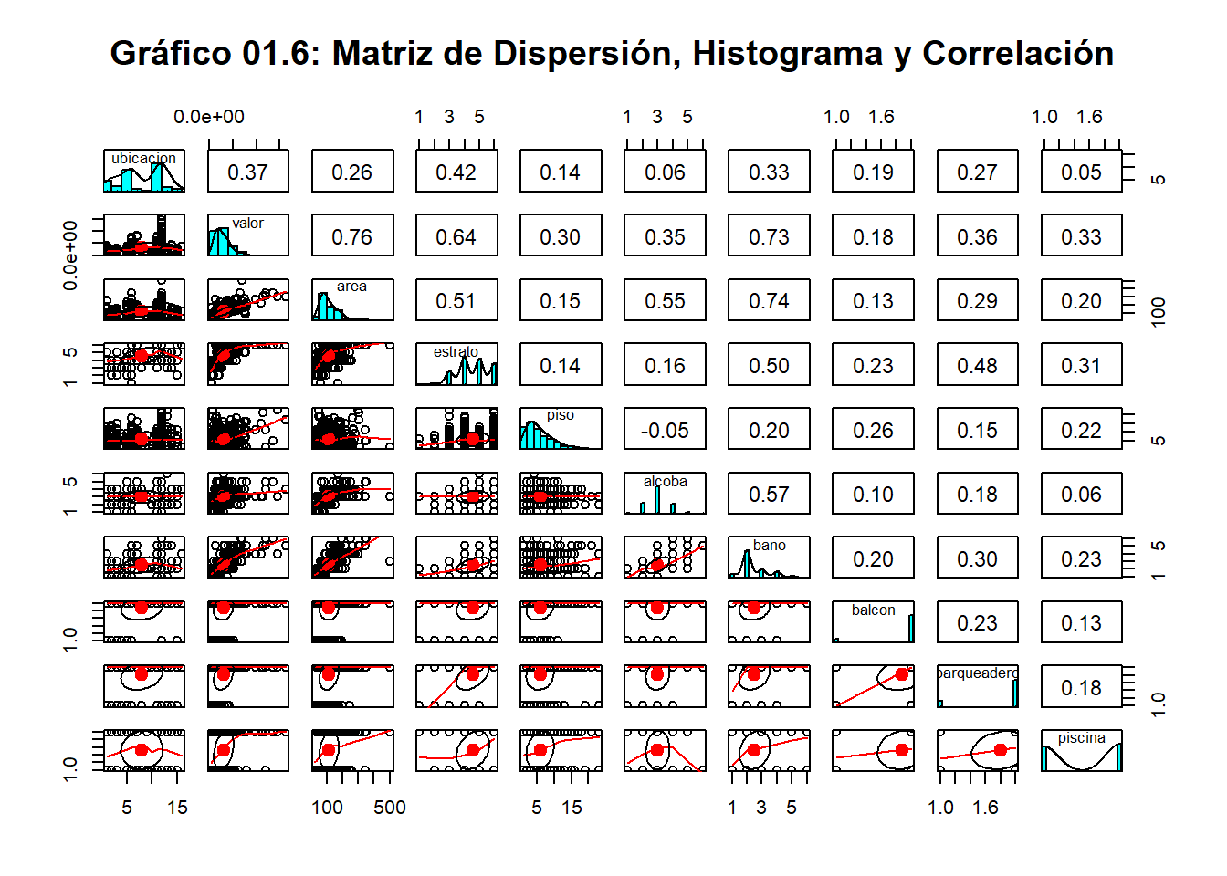
pairs.panels(regresionmult, pch=21,main="Gráfico 01.6: Matriz de Dispersión, Histograma y Correlación")
plot_ly(data = regresionmult, x = ~area, y = ~valor, color = ~as.character(estrato))
## No trace type specified:
##   Based on info supplied, a 'scatter' trace seems appropriate.
##   Read more about this trace type -> https://plot.ly/r/reference/#scatter
## No scatter mode specifed:
##   Setting the mode to markers
##   Read more about this attribute -> https://plot.ly/r/reference/#scatter-mode
plot_ly(data = regresionmult, x = ~area, y = ~valor, color = ~as.character(bano))
## No trace type specified:
##   Based on info supplied, a 'scatter' trace seems appropriate.
##   Read more about this trace type -> https://plot.ly/r/reference/#scatter
## No scatter mode specifed:
##   Setting the mode to markers
##   Read more about this attribute -> https://plot.ly/r/reference/#scatter-mode
regmult=lm(valor~area+estrato+bano,data=regresionmult)
regmult=lm(valor~area+as.character(estrato)+as.character(bano),data=regresionmult)
summary(regmult)
##
## Call:
## lm(formula = valor ~ area + as.character(estrato) + as.character(bano),
##     data = regresionmult)
##
## Residuals:
##        Min         1Q     Median         3Q        Max
## -623485644  -46743126   -2742241   38378645  825692778
##
## Coefficients:
##                          Estimate Std. Error t value Pr(>|t|)
## (Intercept)            -111531079   80689403  -1.382  0.16766
## area                      1270539     140131   9.067  < 2e-16 ***
## as.character(estrato)2  123726868   88375349   1.400  0.16227
## as.character(estrato)3  135691015   80486464   1.686  0.09259 .
## as.character(estrato)4  175083936   80202482   2.183  0.02961 *
## as.character(estrato)5  233535676   80343460   2.907  0.00385 **
## as.character(estrato)6  319990022   80626547   3.969 8.54e-05 ***
## as.character(bano)2      23838088   21646137   1.101  0.27143
## as.character(bano)3      39303396   27234618   1.443  0.14975
## as.character(bano)4     160887597   31407755   5.123 4.67e-07 ***
## as.character(bano)5     208333751   39005080   5.341 1.54e-07 ***
## as.character(bano)6     409734413   67172761   6.100 2.48e-09 ***
## ---
## Signif. codes:  0 '***' 0.001 '**' 0.01 '*' 0.05 '.' 0.1 ' ' 1
##
## Residual standard error: 111400000 on 406 degrees of freedom
## Multiple R-squared:  0.7233, Adjusted R-squared:  0.7158
## F-statistic: 96.49 on 11 and 406 DF,  p-value: < 2.2e-16
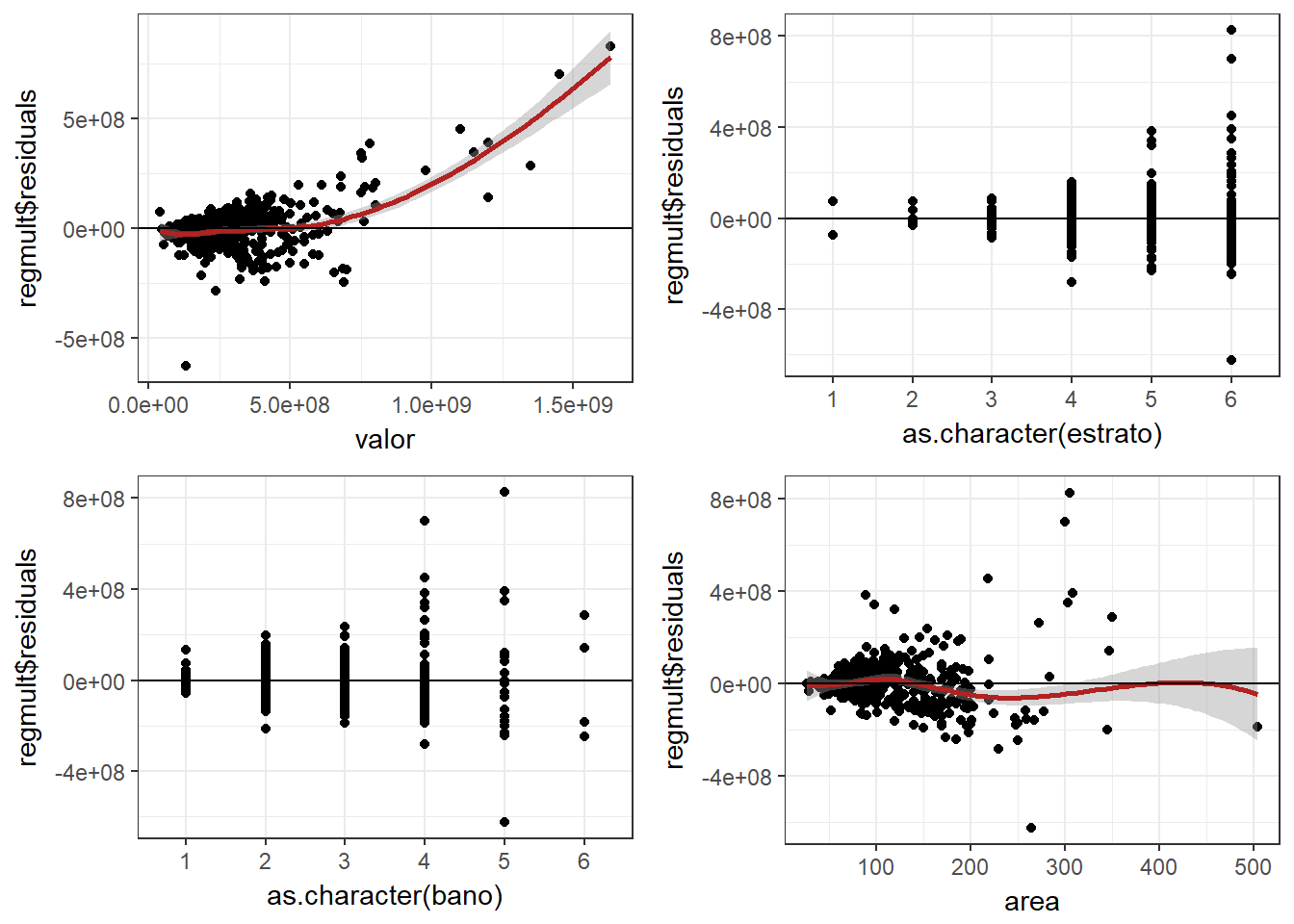
###residuales

plot1 <- ggplot(data = regresionmult, aes(valor, regmult$residuals)) +
    geom_point() + geom_smooth(color = "firebrick") + geom_hline(yintercept = 0) +
    theme_bw()
plot2 <- ggplot(data = regresionmult, aes(as.character(estrato), regmult$residuals)) +
    geom_point() + geom_smooth(color = "firebrick") + geom_hline(yintercept = 0) +
    theme_bw()
plot3 <- ggplot(data = regresionmult, aes(as.character(bano), regmult$residuals)) +
    geom_point() + geom_smooth(color = "firebrick") + geom_hline(yintercept = 0) +
    theme_bw()
plot4 <- ggplot(data = regresionmult, aes(area, regmult$residuals)) +
    geom_point() + geom_smooth(color = "firebrick") + geom_hline(yintercept = 0) +
    theme_bw()
grid.arrange(plot1, plot2, plot3, plot4)
## `geom_smooth()` using method = 'loess'
## `geom_smooth()` using method = 'loess'
## `geom_smooth()` using method = 'loess'
## `geom_smooth()` using method = 'loess'
qqnorm(regmult$residuals)
qqline(regmult$residuals)
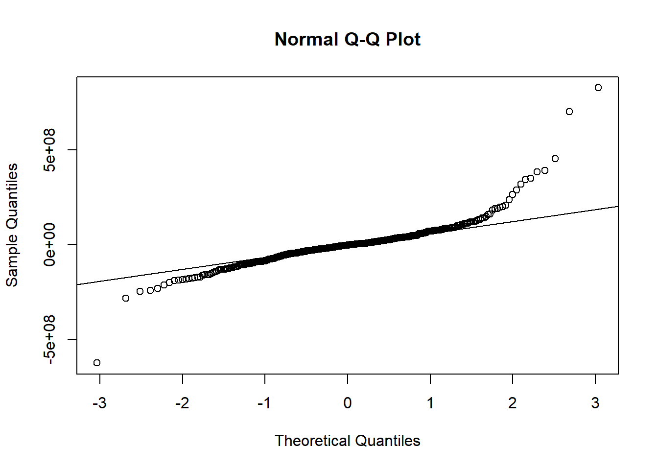
shapiro.test(regmult$residuals)
##
##  Shapiro-Wilk normality test
##
## data:  regmult$residuals
## W = 0.831, p-value < 2.2e-16
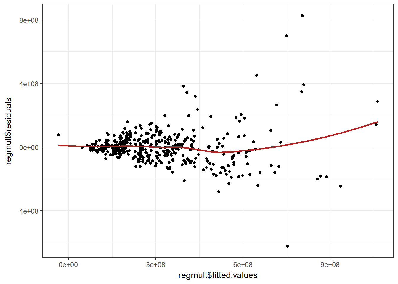
##residuales vs valores ajustados
ggplot(data = regresionmult, aes(regmult$fitted.values, regmult$residuals)) +
geom_point() +
geom_smooth(color = "firebrick", se = FALSE) +
geom_hline(yintercept = 0) +
theme_bw()
## `geom_smooth()` using method = 'loess'